Fundamental OpenCV functions for Image manipulation

In this blog post we will learn fundamental OpenCV functions required for image manipulation tasks. let us dive in….

Image

Image is an array or a matrix of square pixels (picture elements) arranged in columns and rows.

Key terms and types of images

Pixel: Pixels are building blocks of an image. In other words, a pixel is the smallest possible image that can be depicted on the screen.

Binary image: An image that consists of only black & white pixels

Grayscale image: It contains intensity values ranging from a minimum (depicting absolute black) to a maximum (depicting absolute white) and is in between varying shades of gray. Typically, this range is between o & 255.

Color image: The image is composed of three primary colors, Red, Green, Blue. Hence also called an RGB image.

RGB Value: All colors we can see around us can be made by adding red, blue, green components in varying proportions.

Reading, Writing images

import cv2
image = cv2.imread('pic.jpg')
cv2.imwrite('output.jpg',image)

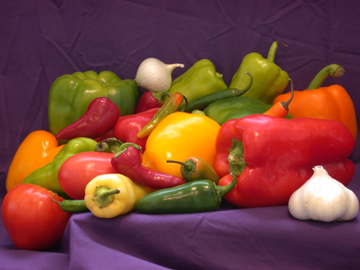
Throughout this blog post, we apply image manipulation techniques on this image.

Changing color spaces

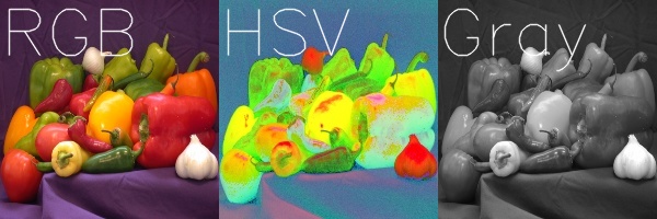
• cvtColor function is used to convert an image from one color space to another

• Some of the popular color conversions such as RGB, BGR, LAB, YaCrCb, and HSV. Since each color space has its own properties, some algorithms or techniques work better in one space than others

• following functions are used to convert from one channel to another channel
  • Converting BGR to RGB: cv2.COLOR_BGR2RGB
  • Converting BGR to GRAY: cv2.COLOR_BGR2GRAY
  • Converting BGR to HSV: cv2.COLOR_BGR2HSV

import cv2
import matplotlib.pyplot as plt
image = cv2.imread('peppers.png')

#show the image
plt.imshow(image)
plt.image()

#Color channels conversion
gray = cv2.cvtColor(image, cv2.COLOR_BGR2GRAY)
hsv = cv2.cvtColor(image, cv2.COLOR_BGR2HSV)

#Saving images
cv2.imwrite('Gray_channel.jpg',gray)
cv2.imwrite('HSV_channel.jpg',hsv)

.

Separating RGB planes

cv2.split function is used to separate the blue, green and red planes

import cv2
import matplotlib.pyplot as plt
image = cv2.imread('peppers.png')
b, g, r=cv2.split(rgb)
#horizontally stacking b, g, r plane images
img1 = cv2.hconcat([b,g,r])
cv2.imwrite('channel_split.jpg',img1)

.

Resizing

Resizing of images is an important concept in computer vision (CV), and machine learning. Images we use for training the model should have the same image dimensions. If we are creating our dataset either by web scraping or from any photo bucket, we can observe the difference in dimensions of an image. In that case, the function cv2.resize will be handy.

The function cv2.resize resizes original image dimensions to required image dimensions.

The following code shows resizing of images in the source folder and saves the resized images in another folder

import cv2
import os,glob
# choose the source path in which original images are stored
src_path = r'C:\opencv_functions\source'
#destination path to save restored images
dst_path = 'C:\opencv_functions\source\dst'
#The glob module used to retrieve the files/pathnames matching with a specified pattern.
#if the images are  ".png" format, replace ".jpg" with ".png"

for fil in glob.glob("*.jpg"):
    #function reads image in the source folder
    image = cv2.imread(fil)
    #cv2.resize(image, (required dimension,(rows, columns)))
    resize = cv2.resize(image,(200,200))
    #saving the resized images in dst_path
    cv2.imwrite(os.path.join(dst_path,fil),resize)
    print(image.shape)
    print(resize.shape)

Other parameters The term Interpolation refers to resize or distort your image from one pixel grid to another. Interpolation works by using known data to estimate values at unknown points. Image interpolation works in two directions, and tries to achieve a best approximation of a pixel’s intensity based on the values at surrounding pixels.

Common interpolation algorithms can be grouped into two categories: adaptive and non-adaptive. Adaptive methods change depending on what they are interpolating, whereas non-adaptive methods treat all pixels equally. Non-adaptive algorithms include: nearest neighbor, bilinear, bicubic, spline, sinc, lanczos and others. Adaptive algorithms include many proprietary algorithms in licensed software such as: Qimage, PhotoZoom Pro and Genuine Fractals.

INTER_NEAREST Interpolation: INTER_NEAREST Interpolation: Duplicate the rows and columns to get the interpolated or zoomed image.

INTER_BILINEAR: Applying a linear interpolation in two directions, thus it gives 4 nearest neighbors, takes their weighted average to produce the output.

INTER_CUBIC: Bicubic interpolation over 4x4 pixels neighbourhood.

let us resize the image say, 20 x 20 and then let’s zoom it 10 times using each interpolation method.

where fx and fy are scale factor along x and y and interpolation flag refers to which method we are going to use. Either you specify (fx, fy) or out_img.size(), OpenCV calculates the other automatically.

import cv2
import matplotlib.pyplot as plt
image= cv2.imread('peppers.png')
resize_1 = cv2.resize(image, (20,20))

#Saving resized image
cv2.imwrite('resize_20_22.jpg', resize_1)

#plot
#plt.imshow('resize_20_22.jpg')
#plt.show()

img = cv2.imread('resize_20_22.jpg')
#Task: let us zoom it 10 times using interpolation method

near_img = cv2.resize(img, None, fx=10, fy=10, interpimglation = cv2.INTER_NEAREST)
cv2.imwrite('near_img.jpg', near_img)

bilinear_img = cv2.resize(img, None, fx=10, fy=10, interpolation = cv2.INTER_LINEAR)
cv2.imwrite('bilinear_img.jpg', bilinear_img)

bicubic_img = cv2.resize(img, None, fx=10, fy=10, interpolation = cv2.INTER_CUBIC)
cv2.imwrite('bicubic_img.jpg', bicubic_img)

.

.

.

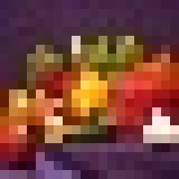Image rotation

Image rotation is a crucial part of machine learning models, if the dataset doesn’t have enough samples, the performance results of the model degrade. By altering images, we can generate a new one. There are many scenarios where rotating the image to various angles can help us gain efficiency in the model.

import cv2
image = cv2.imread('peppers.png')
img_rotate=cv2.rotate(image, cv2.ROTATE_90_CLOCKWISE)
cv2.imwrite('rotate_90.jpg', img_rotate)

.

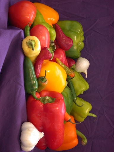Even though the above method is super easy to use, it also restricts us to a few options, we can’t rotate in any angle we want. To have more control over the rotation we can use getRotationMatrix2D

import cv2
image = cv2.imread('peppers.png')


rows, cols = image.shape[:2]
img_rotate=cv2.rotate(image, cv2.ROTATE_90_CLOCKWISE)
cv2.imwrite('rotate_90.jpg', img_rotate)
deg= 45
# (cols/2, rows/2) refers centre rotation, deg- number of degrees to rotate
m = cv2.getRotationMatrix2D((cols/2, rows/2), deg, 1)
image_rotate_degrees = cv2.warpAffine(image, m, (cols, rows))
cv2.imwrite('image_rotate_degrees.jpg',image_rotate_degrees)

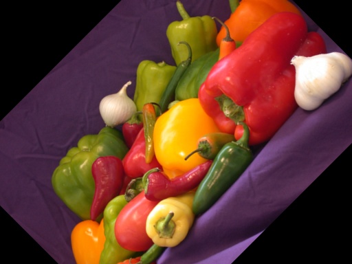
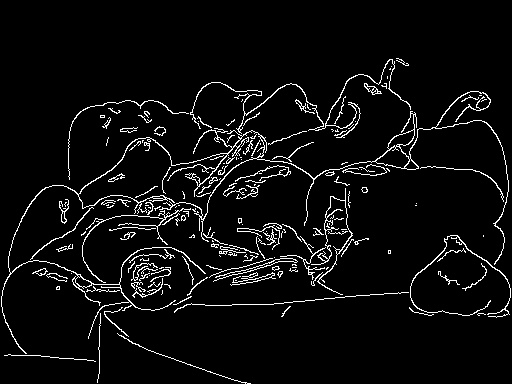
Edge detection

Edges are the points in an image brightness changes sharply or have discontinuities, such discontinuities correspond to :

• Discontintinuities in depth
• Discontinituities in surface orientation
• Changes in material properties
• Variations in scene illumination

import cv2
image_edge = cv2.imread('peppers.png')
edges=cv2.Canny(image,100,200)
cv2.imwrite('edge_detection.jpg',edges)
plt.imshow(edges)
plt.show()