U-Net: Convolutional Networks for Biomedical Image Segmentation- Summarized

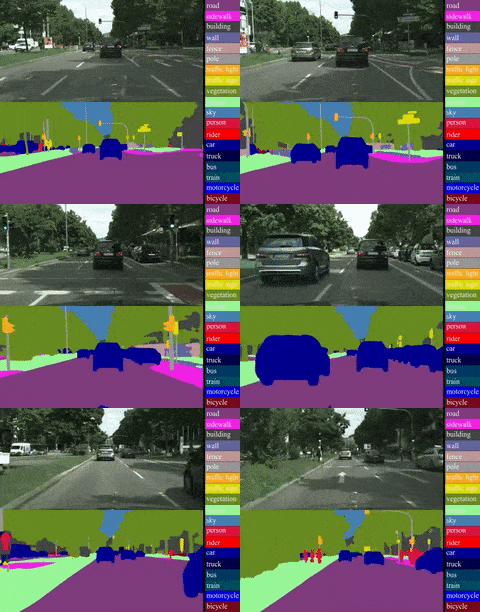
The Use of convolutional networks is on classification tasks, where the output of an image is a single class label. However, in many visual tasks, especially in biomedical image processing, the desired output should include localization. i.e Class label is supposed to be assigned to each pixel (pixel-wise labelling).

Pixel-wise semantic segmentation

Pixel-wise semantic segmentation refers to the process of linking each pixel in an image to a class label. (for more refer my blog post)

.

In this post we will summarize U-Net a fully convolutional networks for Biomedical image segmentation. The architecture of U-Net yields more precise segmentations with less number of images for training data.

Biomedical segmentation with U-Net

.

• U-Net learns segmentation in an end-to-end setting.

• Require less number of images for traning
  • In many visual tasks, especially in biomedical image processing availibility of thousands of training images are usually beyond reach.

• Desired output include localization.

• requires very few-annotated images (approx. 30 per application).

Earlier Approach

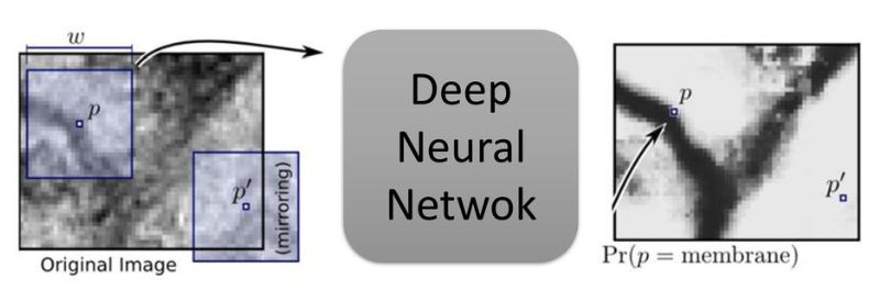
Ciresan et al. trained a network in sliding-window setup to predict the class label of each pixel by providing a local region (patch) around that pixel as input.

.

Advantages

1. The network can localize.

2. The training data in terms of patches is much larger than the number of training images.

Drawbacks

1. It is quite slow because the network must be run separately for each patch, and there is a lot of redundancy due to overlapping patches.

2. There is trade-off between localization and the use of context. Larger patches require more max-pooling layers that reduce the localization accuracy, while small patches allow the network to see only little context.

There was a need of new approach which can do good localization and use of context at the same time.

Fully convolutional neural network (FCN) architecture for semantic segmentation

.

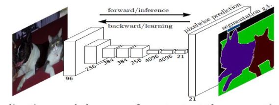
This approach is inspired from the previous work

Main Objectives

1. Localization and the use of context at the same time

2. Input image with any size

3. Added Simple Decoder (Upsampling + conv)

4. Removed Dense Layers.

So Localization and the use of contect at the same time.

U-Net (Modified & Extended Fully convolutional neural network)

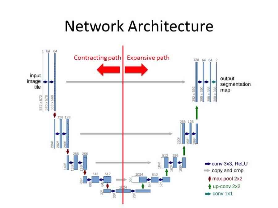
The U-Net architecture is built upon the Fully convolutional Network and modified in a way that it yields better segmentation. Compared to FCN, the two main differences are

1. U-Net is symmetric

2. Skip connections between the downsampling path and the upsampling path apply a concatenation operator instead of a sum. These skip connections intend to provide local information while upsampling. .

U-Net architecture is separated in 3 parts

• The contracting/ downsampling path

• Bottleneck

• The expanding/ upsampling path

Contracting/ downsampling path

The Contracting path is composed of 4 blocks. Each block is composed of

• 3x3 Convolution Layer + activation function (with batch normalization).

• 3x3 Convolution layer + activation function (with batch normalization).

• 2x2 Max Pooling with stride 2 that doubles the number of feature channels.

you can observe that the number of feature maps doubles at each pooling, starting with 64 feature maps for the first block, 128 for the second, and so on.

The purpose of this contracting path is to capture the context of the input image in order to be able to do segmentation.

The coarse contectual information will then be transfered to the upsampling path by means of skip connections.

Bottleneck

This part of the network is between the contraction and expanding paths. The bottleneck is built from simply 2 convolutional layers (with batch normalization), with dropout.

Expanding/ upsampling path

The expanding path is also composed of 4 blocks. Each of these blocks is composed of

• 2x2 up-convolution that halves the number of feature channels.

• Concatenation with the corresponding cropped feature map from the contracting path.

• 3x3 Convolution layer + activation function (with batch normalization)

At the final layer, a 1x1 convolution is used to map each 64 component feature vector to the desired number of classes.

The propose of this expanding path is to enable precise localization combined with contextual information from the contracting path.

U-Net Strategy

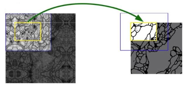
Over-tile strategy for arbitrary large images

.

• Segmentation of the yellow area uses input data of the blue area.

• Raw data extrapolation by mirroring.

The tiling strategy is important to apply the network to large images, since otherwise the resolution would be limited by the GPU memory.

Loss Function

The loss function of U-Net is computed by weighted pixel-wise cross entropy

\[L = \sum_{x\in\Omega}w(x)log(p_{l(x)}(x))\]

where \(p_{l(x)}(x)\) is a softmax of a particular pixel’s true label.

Pixel-wise loss weight

we pre-compute the weight map \(w(x)\) for each ground truth segmentation to

• Force the network to learn the small separation borders that they introduce between touching cells.

• Compensate the different frequency of pixels from a certain class in the training dataset.

\[w(x) = w_c(x) + w_0 exp(-\frac{(d_1(x)+d_2(x))^2}{2\sigma^2})\]

where \(w_c\) is the weight map to balance the class frequencies, \(d_1\) denotes the distance to the border of the nearest cell, and \(d_2\) denotes the distance to the border of the second nearest cell. The authors set \(w_0=10\) and \(\sigma \approx 5\)

Data Augmentation

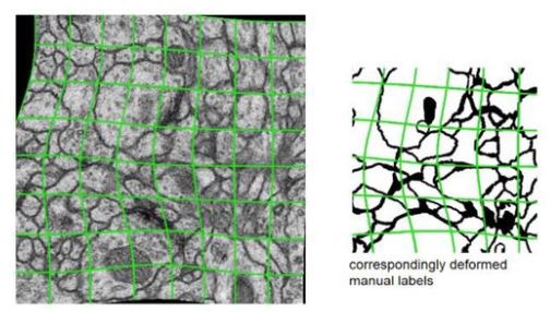
• Random elastic deformation of the training samples.

• shift and rotation invariance of the training samples.

• They use random displacement vectors on 3 by 3 grid.

• The displcement are sampled from gaussian distribution with standard deviationof 10 pixels.

Experiment Results

EM segmentation challenge

ISBI Cell tracking challenge

U-Net Advantages

• Flexible and can be used for any rational image masking task.

• High accuracy (Given proper training, dataset, and training time).

• Doesn’t contain any fully connected layers.

• Faster than the sliding-window (1-sec per image).

• Proven to be very powerful segmentation tool in scenarious with limited data.

• Succeeds to achieve very good performances on different biomedical segmentation applications.

U-net disadvantages

• Larger images need high GPU memory.

• Takes significant amount of time to train (relatively many layer).